Exercise: Day 5 - Expression Analysis with RNA-seq
Get the data
Download the following data of from https://www.dropbox.com/sh/gcsyyf4wumou1gq/AADTP8Z3Vgv7Teja1iEI6ls-a?dl=0
PRAD_raw_counts.txt - Raw counts on 86 matched tumor-normal samples and 55635 genes
PRAD_sample_info.txt - Labels associated to the samples (“Primary Tumor” and “Solid Tissue”)
Load the data into R
Do this by either first downloading the file and providing the local path:
rm(list=ls()) # clean the workspace
setwd("path_to_files") #replace location with local path_to_file
prad_data <- read.table("PRAD_raw_counts.txt",sep="\t",header=T)
RPKM values
Assuming the gene lengths defined below, write a function that, receiving in input the counts from each sample and the gene lengths, calculate the RPKM values
head(prad_data[,1:5])
##          TCGA_HC_8260_11A TCGA_HC_8259_11A TCGA_EJ_7123_11A TCGA_G9_6496_01A TCGA_EJ_7781_01A
## TSPAN6               3829             3990             2770             2666             4454
## TNMD                   10               23               24                5                6
## DPM1                 1555             2108             1987              551             1531
## SCYL3                1096             1598             1477              426             1792
## C1orf112              236              279              307               75              273
## FGR                   222              382              765              203              338
gene_lengths<-rep(c(100,1000),dim(prad_data)[1])[dim(prad_data)[1]]
returnRPKM <- function(counts, gene_lengths) {
....
  return(rpkm)
}

prad_data_rpkm<-apply(prad_data,2,function(x) returnRPKM(x,gene_lengths))

head(prad_data_rpkm[,1:5])
##          TCGA_HC_8260_11A TCGA_HC_8259_11A TCGA_EJ_7123_11A TCGA_G9_6496_01A TCGA_EJ_7781_01A
## TSPAN6         689.840938       602.398597       233.542303       638.641255      666.9722899
## TNMD             1.801622         3.472473         2.023471         1.197752        0.8984809
## DPM1           280.152170       318.259710       167.526555       131.992247      229.2623655
## SCYL3          197.457735       241.261393       124.527791       102.048453      268.3462828
## C1orf112        42.518271        42.122609        25.883569        17.966277       40.8808790
## FGR             39.996001        57.673249        64.498145        48.628723       50.6144216
Data handling and diagnostic plots
A. Starting from the raw count data, filter out the genes characterized by a maximum expression level across the samples which is not above 10 and log2 transform the data, using an offset =1
....

dim(prad_data_filt)
## [1] 29741 86
B. Perform the PCA analysis and plot the first two components, highlighting Primary Tumor vs Solid Tissue Normal classification (NOTE: use pch=19 and col=condition)
samp_info<-read.table("PRAD_sample_info.txt",sep="\t",header=T)
condition<-as.factor(samp_info[,2])
....

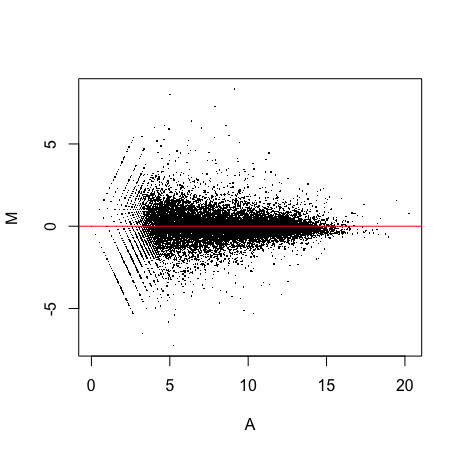
C. Write a function able to display, for a sample given as input, its MA plot versus the “median sample”, i.e. the sample of the median expression values across the genes (NOTE: use the parameter pch=”.” in the plot, and abline to highlight the 0 line)
MAplot<-function(data,n) #n = number indicating the sample
{
....
}

MAplot(prad_data_filt,n=1)
D. Install and load the package “arrayQualityMetrics”, follow the instructions below and look at the resulting report.
source("https://bioconductor.org/biocLite.R")
biocLite("arrayQualityMetrics")
library(arrayQualityMetrics)

condition<-samp_info[,2]
ggt<-data.frame(Group=condition)
row.names(ggt)<-samp_info[,1]
lab<-new("AnnotatedDataFrame",data=ggt)
ddt<-new("ExpressionSet",exprs=as.matrix(prad_data_filt),phenoData=lab)
datx<-prepdata(ddt,intgroup="Group",do.logtransform=FALSE)

arrayQualityMetrics(ddt,outdir="PRAD_raw_counts",intgroup="Group")
Normalization with DESeq2
Install and load the library DESeq2 and use the functions “DESeqDataSetFromMatrix”,”estimateSizeFactors”” and “counts” to obtain the normalized count, starting from the filtered raw count data, NOT log2 transformed. Generate the QC report (using the log2 transformed data plus offset=1) for these data and look how the dignostic plots change with respect to the report obtained from the raw data.
source("https://bioconductor.org/biocLite.R")
biocLite("DESeq2")
library("DESeq2")

ll<-apply(prad_data,1,max)
ind<-which(ll>10)
prad_data_filt<-prad_data[ind,]

condition<-as.factor(samp_info[,2])
ddsMat <- DESeqDataSetFromMatrix(countData = prad_data_filt,DataFrame(condition), ~ condition)
.... #create matnorm

head(matnorm[,1:5])
##          TCGA_HC_8260_11A TCGA_HC_8259_11A TCGA_EJ_7123_11A TCGA_G9_6496_01A
## TSPAN6         4043.35607       3585.40222       1801.94582       5351.86640
## TNMD             10.55982         20.66773         15.61253         10.03726
## DPM1           1642.05241       1894.24258       1292.58713       1106.10592
## SCYL3          1157.35656       1435.95808        960.82093        855.17445
## C1orf112        249.21181        250.70858        199.71024        150.55888
## FGR             234.42806        343.26407        497.64930        407.51271
         TCGA_EJ_7781_01A
TSPAN6        3956.467495
TNMD             5.329772
DPM1          1359.980183
SCYL3         1591.825270
C1orf112       242.504631
FGR            300.243829
condition<-as.character(samp_info[,2])
ggt<-data.frame(Group=condition)
row.names(ggt)<-as.character(samp_info[,1])
lab<-new("AnnotatedDataFrame",data=ggt)
ddt<-new("ExpressionSet",exprs=log2(matnorm+1),phenoData=lab)
datx<-prepdata(ddt,intgroup="Group",do.logtransform=FALSE)

arrayQualityMetrics(ddt,outdir="PRAD_norm_counts",intgroup="Group")
Differential analysis with DESeq2
Firstly, it is better to be sure that the “Solid Tissue Normal” is the first level in the condition factor, so that the default log2 fold changes are calculated as tumor over normal. The function relevel achieves this:
ddsMat$condition <- relevel(dds$condition, "Solid Tissue Normal")
The DESeq2 analysis can now be run with a single call to the function DESeq:
dds <- DESeq(ddsMat)
Calling “results” without any arguments will extract the estimated log2 fold changes and p values:
res <- results(dds)
As res is a DataFrame object, it carries metadata with information on the meaning of the columns:
mcols(res, use.names=TRUE)
## DataFrame with 6 rows and 2 columns
##                       type
##                <character>
## baseMean       intermediate
## log2FoldChange      results
## lfcSE               results
## stat                results
## pvalue              results
## padj                results
##                                                                           description
##                                                                           <character>
## baseMean                                    mean of normalized counts for all samples
## log2FoldChange log2 fold change (MAP): condition Primary Tumor vs Solid Tissue Normal
## lfcSE                  standard error: condition Primary Tumor vs Solid Tissue Normal
## stat                   Wald statistic: condition Primary Tumor vs Solid Tissue Normal
## pvalue              Wald test p-value: condition Primary Tumor vs Solid Tissue Normal
## padj                                                             BH adjusted p-values
The first column, baseMean, is a just the average of the normalized count values, dividing by size factors, taken over all samples. The remaining four columns refer to a specific contrast, namely the comparison of the tumor samples over the normal samples for the factor variable condition. Look at the help page for results.
The column log2FoldChange is the effect size estimate. It tells us how much the gene’s expression seems to have changed due to treatment with dexamethasone in comparison to untreated samples. This value is reported on a logarithmic scale to base 2: for example, a log2 fold change of 1.5 means that the gene’s expression is increased by a multiplicative factor of (2^1.5)≈2.82.
This estimate has an uncertainty associated with it, which is available in the column lfcSE, the standard error estimate for the log2 fold change estimate. DESeq2 performs for each gene a hypothesis test to see whether evidence is sufficient to decide against the null hypothesis that there is no effect of the tumor on the gene and that the observed difference between tumor and control was merely caused by experimental variability (i.e., the type of variability that you can just as well expect between different samples in the same condition group). As usual in statistics, the result of this test is reported as a p value, and it is found in the column pvalue.
To look at the genes with a p value below 0.05:
sum(res$pvalue < 0.05, na.rm=TRUE)
## [1] 16044
Now, assume for a moment that the null hypothesis is true for all genes, i.e., no gene is affected by the condition tumor vs normal. Then, by the definition of p value, we expect up to 5% of the genes to have a p value below 0.05. However, we have more genes selected than the 5% of the total. DESeq2 uses the Benjamini-Hochberg (BH) adjustment as described in the base R p.adjust function in order to decrease the number of false positives.
A. Look at the number of genes with adjusted p-value below 5%.
....
## [1] 14369
To select the number of significant genes:
resSig <- subset(res, padj < 0.05)
B. Use DEseq2 function plotMA and use a threshold for alpha = 0.05

Final Exercise Download the GBM data from the same link reported above and repeat the pipeline. Use DESeq2 with the condition tumor vs. normal and try to combine this condition with the age or the gender as in the example:
ddsMat <- DESeqDataSetFromMatrix(countData = gbm_data_filt,.... ~ condition+gender)