Exercise: Day 4 - Introduction to Unix, HPC, and Linear Algebra
Unix and Orchestra
Exercise 1: “Quality trimming on 6 Fastq files, in serial with multithreading”
- Log into Orchestra using Terminal or Putty or Git BASH
- Start an interactive session with a single core
- Change directories into the
~/unix-intro/, and move thetrimmomatic-serial.lsffile/script from theotherdirectory to your current directory (~/unix-intro/) - Open the script with
nano - Modify the LSF (bsub) directives to use only 4 cores
- Add a bsub directive to make sure that you get an email when the job completes
- Submit the script to the LSF queue using
bsub(Hint: Job submissions use special syntax and justbsub scriptname.lsfwill not work) - Once submitted, immediately check the status of your job. How many jobs do you see running? Is there a difference in the “Queue” on which they are running?
- When the job is completed it will create a new directory with new files: What is the name of the new directory? How many new files and directories were created within it?
- List only those files that end in
.zip,
Exercise 2: “Quality trimming on 6 Fastq files, in parallel with multithreading”
- Check and make sure you have an interactive session going and also that you are in the
~/unix-intro/directory. - Copy over the
trimmomatic-on-input-file.shandtrimmomatic-multithreaded.shfiles from theotherdirectory to your current directory - Use
nanoto open thetrimmomatic-multithreaded.shfile and make note of the bsub submission command in it. Is this a file that can be submitted to LSF usingbsub < scriptname? - Run
trimmomatic-multithreaded.shusing sh instead ofbsub < - How many job submission notification did you get?
- Once submitted, immediately check the status of your jobs. How many are running and how many are pending?
- Once again, when the job is complete a new directory with new files will be created. Use
ls -lto determine if the same output was generated for both. - What do you think the advantage is of running the job(s) this way as compared to Exercise 1?
Principal Components Analysis
Get the data
We will be using the same expression data as for the Day 1 exercises. Instructions for loading that dataset are copied below:
Download the following data of from https://tcga-data.nci.nih.gov/docs/publications/gbm_exp/
unifiedScaledFiltered.txt - Filtered unified gene expression estimate for 202 samples and 1740 genes
Load the data into R
Do this by either first downloading the file and providing the local path:
#replace location with local path_to_file
my_data <- read.table("../data/unifiedScaledFiltered.txt",sep="\t",header=1)
..or by reading the file directly from the remote location:
#source("https://bioconductor.org/biocLite.R") #run if necessary
#biocLite("curl") #run if necessary
library(curl)
my_data <- read.table(curl("https://tcga-data.nci.nih.gov/docs/publications/gbm_exp/unifiedScaledFiltered.txt"),sep="\t",header=1)
A. Before we get started, we should examine the range of our gene expression vectors. Which genes have the highest and lowest mean expression? What about the variances of the genes? What does this tell you about the data?
B. Perform a PCA on the GMB expression data, paying special attention to centering and scaling data (hint: what are the default options for the R function “prcomp”?) How many PCs do you find?
C. What proportion of total variance is explained by the first PC? What proportion of total variance is explained by the first 10 PCs?
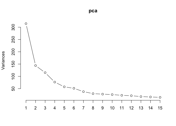
D. Plot the first fifteen principal components by variance. How many should be retained?

E. What genes have the highest absolute loading values for the first principal component? For the second component? Would you expect to find the same genes with the highest loadings for the first and second PCs?
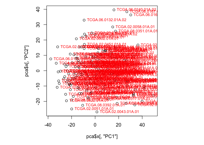
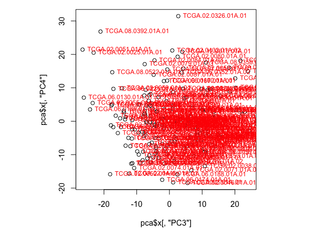
F. Create a scatterplot of the values for the first and second PCs. Label the points with the sample names, and note which samples stand out. Does this change if you plot a different set of components? (Hint: Use plot() to create a scatterplot and text() to add labels to those points)

