
WGCNA: Weighted gene co-expression network analysis
This code has been adapted from the tutorials available at WGCNA website
Getting started: in order to run R on Orchestra, we will first connect to an interactive queue
# bsub -n 2 -Is -q interactive bash
# git clone https://github.com/hms-dbmi/scw.git
# cd scw/scw2015
# source setup.sh
# R
Loading WGCNA library, and settings to allow parallel execution. Please note that WGCNA and dependencies have been already installed for you.
library(WGCNA)
## Loading required package: dynamicTreeCut
## Loading required package: fastcluster
##
## Attaching package: 'fastcluster'
##
## The following object is masked from 'package:stats':
##
##     hclust
##
## Loading required package: DBI
##
##
## Attaching package: 'WGCNA'
##
## The following object is masked from 'package:stats':
##
##     cor
library("flashClust")
##
## Attaching package: 'flashClust'
##
## The following object is masked from 'package:fastcluster':
##
##     hclust
##
## The following object is masked from 'package:stats':
##
##     hclust
options(stringsAsFactors = FALSE);
enableWGCNAThreads()
Loading the data; WGCNA requires genes be given in the columns
load("/groups/pklab/scw/scw2015/data/varinfo.RData");
mydata=varinfo$mat;
dim(mydata)
## [1] 12831 90
gene.names=names(sort(varinfo$arv,decreasing=T));
mydata.trans=t(mydata);
For the purpose of this exercise, we focus on a smaller set of genes:
n=500;
datExpr=mydata.trans[,gene.names[1:n]];
SubGeneNames=gene.names[1:n];
Choosing a soft-threshold power: a tradeoff between scale free topology and mean connectivity
powers = c(c(1:10), seq(from = 12, to=20, by=2));
sft=pickSoftThreshold(datExpr,dataIsExpr = TRUE,powerVector = powers,corFnc = cor,corOptions = list(use = 'p'),networkType = "signed")
##    Power SFT.R.sq  slope truncated.R.sq mean.k. median.k. max.k.
## 1      1   0.0742 -7.290          0.940 266.000  265.0000 287.00
## 2      2   0.0580  2.940          0.931 146.000  147.0000 166.00
## 3      3   0.0106 -0.818          0.938  83.100   83.2000 105.00
## 4      4   0.1330 -1.980          0.984  48.500   47.7000  70.00
## 5      5   0.2770 -2.120          0.961  29.100   28.0000  50.00
## 6      6   0.5250 -2.360          0.941  17.900   16.7000  36.90
## 7      7   0.7130 -2.420          0.946  11.300   10.1000  27.90
## 8      8   0.8410 -2.240          0.956   7.250    6.1900  21.50
## 9      9   0.9110 -2.150          0.972   4.780    3.8100  16.80
## 10    10   0.9280 -2.060          0.940   3.210    2.3800  13.40
## 11    12   0.9530 -1.870          0.950   1.540    0.9700   9.00
## 12    14   0.9510 -1.740          0.938   0.795    0.4050   6.48
## 13    16   0.9590 -1.650          0.948   0.440    0.1750   4.84
## 14    18   0.9270 -1.570          0.907   0.258    0.0779   3.72
## 15    20   0.9140 -1.480          0.893   0.160    0.0353   2.91
# Plot the results
sizeGrWindow(9, 5)
par(mfrow = c(1,2));
cex1 = 0.9;

# Scale-free topology fit index as a function of the soft-thresholding power
plot(sft$fitIndices[,1], -sign(sft$fitIndices[,3])*sft$fitIndices[,2],xlab="Soft Threshold (power)",ylab="Scale Free Topology Model Fit, signed R^2",type="n", main = paste("Scale independence"));
text(sft$fitIndices[,1], -sign(sft$fitIndices[,3])*sft$fitIndices[,2],labels=powers,cex=cex1,col="red");

# Red line corresponds to using an R^2 cut-off
abline(h=0.80,col="red")

# Mean connectivity as a function of the soft-thresholding power
plot(sft$fitIndices[,1], sft$fitIndices[,5],xlab="Soft Threshold (power)",ylab="Mean Connectivity", type="n",main = paste("Mean connectivity"))
text(sft$fitIndices[,1], sft$fitIndices[,5], labels=powers, cex=cex1,col="red")
Generating adjacency and TOM similarity matrices based on the selected softpower
softPower = 8;

#calclute the adjacency matrix
adj= adjacency(datExpr,type = "signed", power = softPower);

#turn adjacency matrix into a topological overlap matrix (TOM) to minimize the effects of noise and spurious associations
TOM=TOMsimilarityFromExpr(datExpr,networkType = "signed", TOMType = "signed", power = softPower);
## TOM calculation: adjacency..
## ..will use 11 parallel threads.
##  Fraction of slow calculations: 0.000000
## ..connectivity..
## ..matrix multiplication..
## ..normalization..
## ..done.
colnames(TOM) =rownames(TOM) =SubGeneNames
dissTOM=1-TOM
Module detection
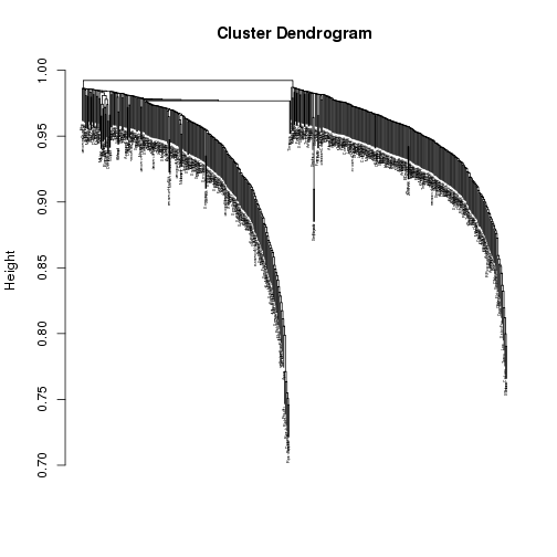
#hierarchical clustering of the genes based on the TOM dissimilarity measure
geneTree = flashClust(as.dist(dissTOM),method="average");

#plot the resulting clustering tree (dendrogram)
plot(geneTree, xlab="", sub="",cex=0.3);
# Set the minimum module size
minModuleSize = 20;

# Module identification using dynamic tree cut

dynamicMods = cutreeDynamic(dendro = geneTree,  method="tree", minClusterSize = minModuleSize);
#dynamicMods = cutreeDynamic(dendro = geneTree, distM = dissTOM, method="hybrid", deepSplit = 2, pamRespectsDendro = FALSE, minClusterSize = minModuleSize);

#the following command gives the module labels and the size of each module. Lable 0 is reserved for unassigned genes
table(dynamicMods)
## dynamicMods
##   0   1   2
##  74 226 200
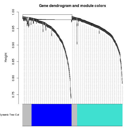
#Plot the module assignment under the dendrogram; note: The grey color is reserved for unassigned genes
dynamicColors = labels2colors(dynamicMods)
table(dynamicColors)
## dynamicColors
##      blue      grey turquoise
##       200        74       226
plotDendroAndColors(geneTree, dynamicColors, "Dynamic Tree Cut", dendroLabels = FALSE, hang = 0.03, addGuide = TRUE, guideHang = 0.05, main = "Gene dendrogram and module colors")
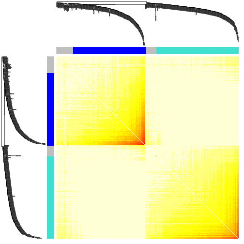
#set the diagonal of the dissimilarity to NA
diag(dissTOM) = NA;

#Visualize the Tom plot. Raise the dissimilarity matrix to a power  to bring out the module structure
sizeGrWindow(7,7)
TOMplot(dissTOM^4, geneTree, as.character(dynamicColors))
Extract modules
module_colors= setdiff(unique(dynamicColors), "grey")
for (color in module_colors){
    module=SubGeneNames[which(dynamicColors==color)]
    write.table(module, paste("module_",color, ".txt",sep=""), sep="\t", row.names=FALSE, col.names=FALSE,quote=FALSE)

}
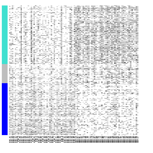
Look at expression patterns of these genes, as they are clustered
module.order <- unlist(tapply(1:ncol(datExpr),as.factor(dynamicColors),I))
m<-t(t(datExpr[,module.order])/apply(datExpr[,module.order],2,max))
heatmap(t(m),zlim=c(0,1),col=gray.colors(100),Rowv=NA,Colv=NA,labRow=NA,scale="none",RowSideColors=dynamicColors[module.order])
We can now look at the module gene listings and try to interpret their functions; for instance using http://amigo.geneontology.org/rte
WGCNA has many more features, such as quantifying module similarity by eigengene correlation, etc. For details, please visit WGCNA website.