
WGCNA: Weighted gene co-expression network analysis
This code has been adapted from the tutorials available at WGCNA website. For the installation and more detailed analysis, please visit the website.
Getting started: in order to run R on Orchestra, we will first connect to an interactive queue
# bsub -n 2 -Is -q interactive bash
# git clone https://github.com/hms-dbmi/scw.git
# cd scw/scw2016
# source setup.sh
# R
Loading WGCNA library, and settings to allow parallel execution. Please note that WGCNA and dependencies have been already installed for you.
library(WGCNA)
library("flashClust")
options(stringsAsFactors = FALSE);
#enableWGCNAThreads()
disableWGCNAThreads()
Loading the data; WGCNA requires genes be given in the columns. For the purpose of this exercise, we focus on a smaller set of n=500 most variable/over-dispersed genes:
load('data/varinfo.RData');
mydata=varinfo$mat;
dim(mydata)

## [1] 12453   224

gene.names=names(sort(varinfo$arv,decreasing=T));
mydata.trans=t(mydata);

n=500;
datExpr=mydata.trans[,gene.names[1:n]];
SubGeneNames=gene.names[1:n];
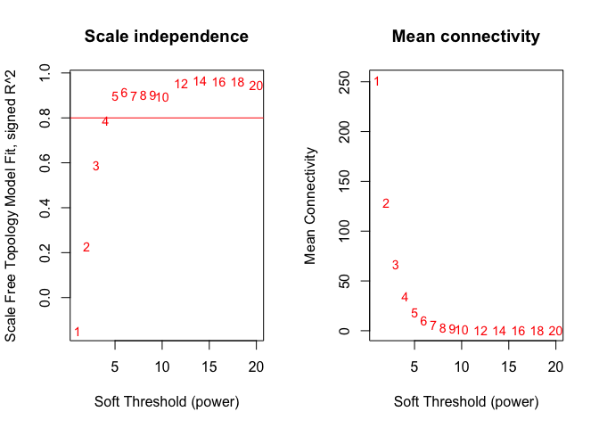
Choosing a soft-threshold power: a tradeoff between scale free topology and mean connectivity
powers = c(c(1:10), seq(from = 12, to=20, by=2));
sft=pickSoftThreshold(datExpr,dataIsExpr = TRUE,powerVector = powers,corFnc = cor,corOptions = list(use = 'p'),networkType = "signed")

##    Power SFT.R.sq  slope truncated.R.sq  mean.k. median.k. max.k.
## 1      1    0.147  27.10          0.939 252.0000  2.51e+02 259.00
## 2      2    0.229 -11.10          0.620 129.0000  1.28e+02 141.00
## 3      3    0.590  -9.73          0.598  66.5000  6.55e+01  81.80
## 4      4    0.786  -7.17          0.728  35.0000  3.38e+01  50.20
## 5      5    0.899  -5.48          0.881  18.7000  1.76e+01  32.60
## 6      6    0.915  -4.17          0.922  10.2000  9.19e+00  22.40
## 7      7    0.899  -3.26          0.930   5.6600  4.83e+00  16.00
## 8      8    0.901  -2.66          0.910   3.2300  2.56e+00  12.00
## 9      9    0.903  -2.22          0.932   1.9000  1.36e+00   9.22
## 10    10    0.896  -1.93          0.924   1.1600  7.25e-01   7.27
## 11    12    0.954  -1.60          0.966   0.4820  2.10e-01   4.91
## 12    14    0.968  -1.41          0.964   0.2330  6.26e-02   3.52
## 13    16    0.960  -1.28          0.949   0.1290  1.91e-02   2.60
## 14    18    0.961  -1.21          0.953   0.0778  5.98e-03   1.95
## 15    20    0.947  -1.15          0.933   0.0501  1.88e-03   1.48

# Plot the results
# sizeGrWindow(9, 5)
par(mfrow = c(1,2));
cex1 = 0.9;

# Scale-free topology fit index as a function of the soft-thresholding power
plot(sft$fitIndices[,1], -sign(sft$fitIndices[,3])*sft$fitIndices[,2],xlab="Soft Threshold (power)",ylab="Scale Free Topology Model Fit, signed R^2",type="n", main = paste("Scale independence"));
text(sft$fitIndices[,1], -sign(sft$fitIndices[,3])*sft$fitIndices[,2],labels=powers,cex=cex1,col="red");

# Red line corresponds to using an R^2 cut-off
abline(h=0.80,col="red")

# Mean connectivity as a function of the soft-thresholding power
plot(sft$fitIndices[,1], sft$fitIndices[,5],xlab="Soft Threshold (power)",ylab="Mean Connectivity", type="n",main = paste("Mean connectivity"))
text(sft$fitIndices[,1], sft$fitIndices[,5], labels=powers, cex=cex1,col="red")
Generating adjacency and TOM similarity matrices based on the selected softpower
softPower = 5;

#Calclute the adjacency matrix
adj= adjacency(datExpr,type = "signed", power = softPower);

#Turn adjacency matrix into a topological overlap matrix (TOM) to minimize the effects of noise and spurious associations
TOM=TOMsimilarityFromExpr(datExpr,networkType = "signed", TOMType = "signed", power = softPower);

## TOM calculation: adjacency..
## adjacency: replaceMissing: 0
## ..will not use multithreading.
##  Fraction of slow calculations: 0.000000
## ..connectivity..
## ..matrix multiplication..
## ..normalization..
## ..done.

colnames(TOM) =rownames(TOM) =SubGeneNames
dissTOM=1-TOM
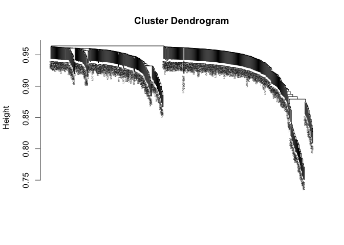
Module detection
#Hierarchical clustering of the genes based on the TOM dissimilarity measure
geneTree = flashClust(as.dist(dissTOM),method="average");

#Plot the resulting clustering tree (dendrogram)
plot(geneTree, xlab="", sub="",cex=0.3);
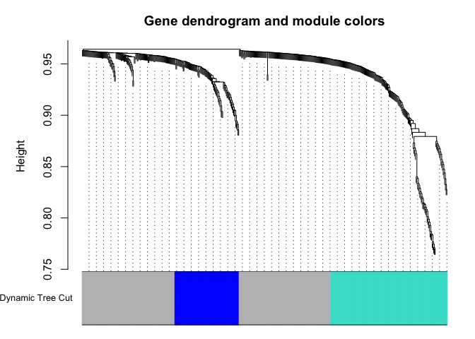
# Set the minimum module size
minModuleSize = 20;

# Module identification using dynamic tree cut, you can also choose the hybrid method

dynamicMods = cutreeDynamic(dendro = geneTree,  method="tree", minClusterSize = minModuleSize);
#dynamicMods = cutreeDynamic(dendro = geneTree, distM = dissTOM, method="hybrid", deepSplit = 2, pamRespectsDendro = FALSE, minClusterSize = minModuleSize);

#Get the module labels and the size of each module. Lable 0 is reserved for unassigned genes
table(dynamicMods)

## dynamicMods
##   0   1   2
## 253 159  88

#Plot the module assignment under the dendrogram; note: The grey color is reserved for unassigned genes
dynamicColors = labels2colors(dynamicMods)
table(dynamicColors)

## dynamicColors
##      blue      grey turquoise
##        88       253       159

plotDendroAndColors(geneTree, dynamicColors, "Dynamic Tree Cut", dendroLabels = FALSE, hang = 0.03, addGuide = TRUE, guideHang = 0.05, main = "Gene dendrogram and module colors")
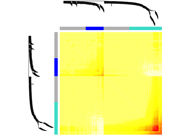
#Set the diagonal of the dissimilarity to NA
diag(dissTOM) = NA;

#Visualize the Tom plot. Raise the dissimilarity matrix to a power  to bring out the module structure
#sizeGrWindow(7,7)
TOMplot(dissTOM^4, geneTree, as.character(dynamicColors))
Extract modules
module_colors= setdiff(unique(dynamicColors), "grey")
for (color in module_colors){
    module=SubGeneNames[which(dynamicColors==color)]
    write.table(module, paste("module_",color, ".txt",sep=""), sep="\t", row.names=FALSE, col.names=FALSE,quote=FALSE)

}
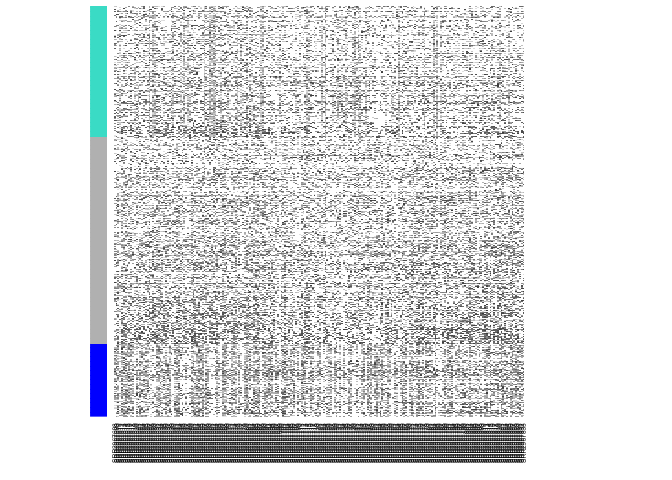
Look at expression patterns of these genes, as they are clustered
module.order <- unlist(tapply(1:ncol(datExpr),as.factor(dynamicColors),I))
m<-t(t(datExpr[,module.order])/apply(datExpr[,module.order],2,max))
heatmap(t(m),zlim=c(0,1),col=gray.colors(100),Rowv=NA,Colv=NA,labRow=NA,scale="none",RowSideColors=dynamicColors[module.order])
We can now look at the module gene listings and try to interpret their functions; for instance using http://amigo.geneontology.org/rte
WGCNA has many more features, such as quantifying module similarity by eigengene correlation, etc. For details, please visit WGCNA website.