
Loading count data
In this section of the tutorial we will be using R to analyse count data of the type generated in the previous tutorial. First we will change directories and start up an instance of R:
$ cd ~/scw/scw2015/differential_expression
$ R
We can now read in our table of counts using the following R commands:
counts <- read.delim("~/scw/scw2015/alignment/subset/combined.counts",skip=0,header=T,sep="\t",stringsAsFactors=F,row.names=1)
Examining the dimensionality of this matrix via the command dim(counts), we can see that there are 23,337 genes detected (rows in the matrix), and 4 cells.
In order to analyse a larger dataset, we will load the counts for the ES/MEF mouse dataset of Islam et al., which contains 48 embyronic stem (ES) cells, and 44 mouse embryonic fibroblast (MEF) cells. For efficiency, this table has been saved as a compressed .RData file.
load("ES_MEF_raw.RData")
# clean up column (cell) names
colnames(counts) <- gsub("L139_Sample(\\d+).counts","\\1",colnames(counts))
colnames(counts)[1:10]
##  [1] "MEF_54" "ESC_47" "MEF_61" "MEF_67" "ESC_19" "MEF_91" "MEF_62"
##  [8] "ESC_20" "ESC_13" "MEF_70"
The rows of the counts data frame represent genes, and the columns represent cells. However, the genes in our count file are named according to their Ensembl ID. In order to map these IDs to more informative gene names, we can use the R interface to BioMart.
We will not run this procedure during this session, so as to avoid overloading the servers with multiple simultaneous requests, but this is how it might be done:
library(biomaRt)
mart <- useMart(biomart = 'ensembl', dataset = 'mmusculus_gene_ensembl')
bm.query <- getBM(values=rownames(counts),attributes=c("ensembl_gene_id", "external_gene_name"),filters=c("ensembl_gene_id"),mart=mart)
genes <- list(ids=rownames(counts),names=bm.query[match(rownames(counts), bm.query$ensembl_gene_id),]$external_gene_name)
Gene identifiers
Due to the reasons mentioned above, we will simply read in the map from Ensembl IDs to gene names from a saved table
load("gene_name_map.RData")
The row names of the count table can then be set to these gene names:
rownames(counts) <- make.unique(as.character(genes$names))
Cell identifiers
The identities of the different cells are known in this case, and we can obtain this information from the first three characters of the column labels:
cell.labels <- substr(colnames(counts),0,3)
The dataset contains some cells that were used as negative controls, so we will remove these before further analysis:
counts <- counts[-which(cell.labels=="EMP")]
cell.labels <- cell.labels[-which(cell.labels=="EMP")]
We will also reorder the cells so that the ES cells (columns) are all in the first half of the matrix, to help with visualisation later:
counts <- cbind(counts[,cell.labels=="ESC"],counts[,cell.labels=="MEF"])
cell.labels <- substr(colnames(counts),0,3)
Preliminary examination of the dataset
We can then examine some features of the dataset:
length(counts[,1]) # number of genes
## [1] 39017
length(cell.labels) # number of cells
## [1] 92
nES <- sum(cell.labels=="ESC") # number of ES cells
nMEF <- sum(cell.labels=="MEF") # number of MEF cells
A factor object can be defined to index the different cell types.
groups <- factor(cell.labels,levels=c("ESC","MEF"))
table(groups)
## groups
## ESC MEF
##  48  44
Before proceeding, we will restrict our attention to those genes that had non-zero expression:
counts <- counts[rowSums(counts)>0,]
nGenes <- length(counts[,1])
We’ll also save the full cleaned up count matrix for use in subsequent analyses:
save(counts,file="counts.RData")
Let’s examine the effective library size (estimated by the average read count per gene) for the different cells.
coverage <- colSums(counts)/nGenes
ord <- order(groups)
bar.positions <- barplot(coverage[ord],col=groups[ord],xaxt='n',ylab="Counts per gene")
axis(side=1,at=c(bar.positions[nES/2],bar.positions[nES+nMEF/2]),labels=c("ESC","MEF"),tick=FALSE)
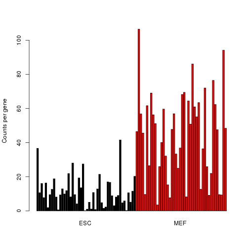
We can see that on average the expression is higher for the MEF cells. We’ll filter out those cells with very low coverage
counts <- counts[,coverage>1]
cell.labels <- cell.labels[coverage>1]
groups <- factor(cell.labels,levels=c("ESC","MEF"))
coverage <- coverage[coverage>1]
nCells <- length(cell.labels)
We can use a violin plot to visualize the distributions of the normalized counts for the most highly expressed genes.
counts.norm <- t(apply(counts,1,function(x) x/coverage)) # simple normalization method
top.genes <- tail(order(rowSums(counts.norm)),10)
expression <- log2(counts.norm[top.genes,]+1) # add a pseudocount of 1
library(caroline)
violins(as.data.frame(t(expression)),connect=c(),deciles=FALSE,xlab="",ylab="log2 expression")
## Loading required package: sm
## Package 'sm', version 2.2-5.4: type help(sm) for summary information
## Loading required package: MASS
##
## Attaching package: 'MASS'
##
## The following object is masked from 'package:sm':
##
##     muscle
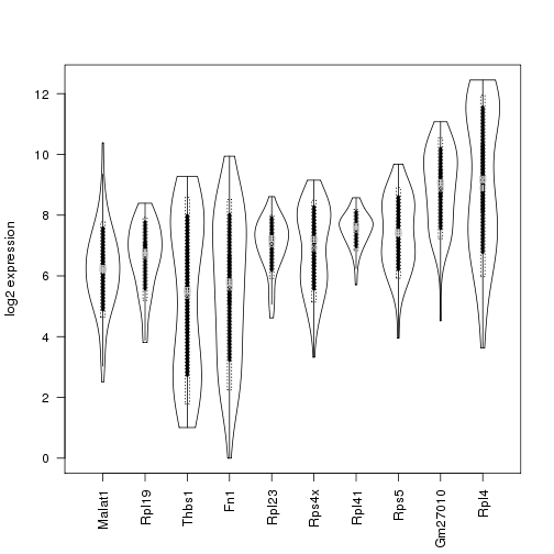
Some of these genes show a clear bimodal pattern of expression, indicating the presence of two subpopulations of cells.
Negative binomial model for counts
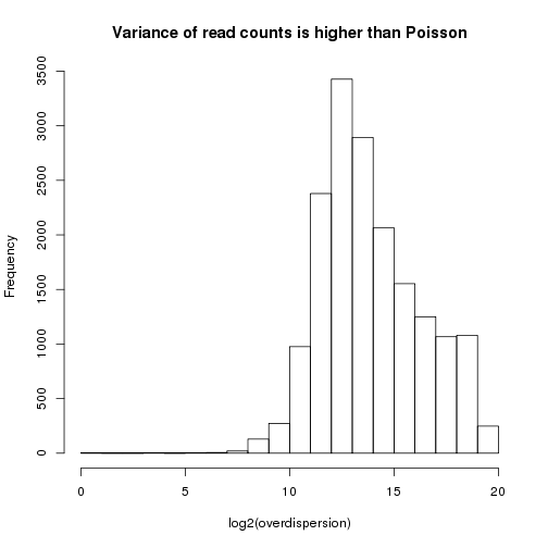
Perhaps the simplest statistical model for count data is the Poisson, which has only one parameter. Under a Poisson model, the variance of the expression for a particular gene is equal to its mean expression. However, due to a variety of types of noise (both biological and technical), a better fit for read count data is usually obtained by using a negative binomial model, for which the variance can be written as:
variance = mean + overdispersion x mean^2
Since the overdispersion is a positive number, the variance under the negative binomial model is always higher than for the Poisson.
On our dataset, the overdispersion is clearly greater than zero for almost all genes, suggesting that the negative binomial will indeed be a better fit:
means <- apply(counts.norm,1,mean)
excess.var <- apply(counts,1,var)-means
excess.var[excess.var < 0] <- NA
overdispersion <- excess.var / means^2
hist(log2(overdispersion),main="Variance of read counts is higher than Poisson")
Running DESeq
library(DESeq)
Several of the steps in the following analyses takes around 5 minutes to run on the full 92-cell dataset, using 2 cores on Orchestra. In order to save time for the purposes of this tutorial session, we will work with a subset of the data, sampling 20 cells from each of the groups:
es.cell.subset <- which(groups=="ESC")[(1:20)*2]
mef.cell.subset <- which(groups=="MEF")[(1:20)*2]
cell.subset <- c(es.cell.subset,mef.cell.subset)
counts <- counts[,cell.subset]
cell.labels <- cell.labels[cell.subset]
groups <- factor(cell.labels,levels=c("ESC","MEF"))
nCells <- length(cell.labels)
First we will use our count and groups objects to create a DESeq CountDataSet object:
cds <- newCountDataSet(counts, groups)
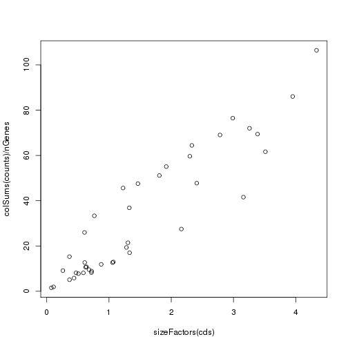
DESeq estimates size factors to measure the library size for each cell.
cds <- estimateSizeFactors(cds)
Generally the estimated size factors are linearly related to the average read count per gene (coverage), but are estimated using a more robust method:
plot(sizeFactors(cds),colSums(counts)/nGenes)
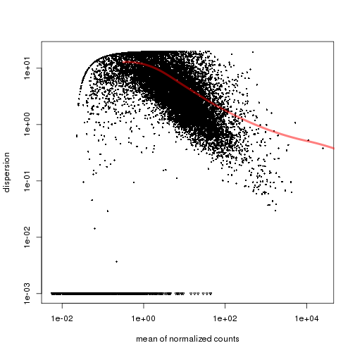
Estimating the overdispersion
In order to compute $p$-values for differential expression, DESeq requires an estimate of the overdispersion for each gene. Since we have $40$ cells in total, we may wish to rely on the empirical estimates of the dispersion:
cds <- estimateDispersions(cds, sharingMode="gene-est-only")
## Warning in .local(object, ...): in estimateDispersions: sharingMode=='gene-
## est-only' will cause inflated numbers of false positives unless you have
## many replicates.
In cases where the empirical estimates may not be so reliable (e.g. when there are very few cells), we can pool information from the other cells in each group in order to obtain a more robust estimator for the dispersion
cds.pooled <- estimateDispersions(cds, method="per-condition",fitType="local")
# check the fit
plotDispEsts(cds.pooled,name="ESC")
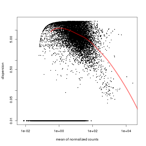
plotDispEsts(cds.pooled,name="MEF")
Differential expression analysis
We are now ready to carry out the differential expression analysis.
de.test <- nbinomTest(cds, "ESC", "MEF")
We will also repeat the analysis using the pooled estimates for the dispersion parameters, to see what kind of difference this makes to the results:
de.test.pooled <- nbinomTest(cds.pooled, "ESC", "MEF")
We can then extract the top differentially expressed genes, using a false discovery rate of $0.05$:
find.significant.genes <- function(de.result,alpha=0.05) {
  # filter out significant genes based on FDR adjusted p-values
  filtered <- de.result[(de.result$padj < alpha) & !is.infinite(de.result$log2FoldChange) & !is.nan(de.result$log2FoldChange),]
  # order by p-value, and print out only the gene name, mean count, and log2 fold change
  sorted <- filtered[order(filtered$pval),c(1,2,6)]
}
de.genes <- find.significant.genes(de.test)
de.genes.pooled <- find.significant.genes(de.test.pooled)
This procedure pulls out a lot of genes as differentially expressed:
length(de.genes[,1])
## [1] 2974
length(de.genes.pooled[,1])
## [1] 778
Examining differentially expressed genes
We can examine the top $15$ of these
head(de.genes.pooled,n=15)
##                   id    baseMean log2FoldChange
## 11228         Dppa5a   630.24357      -6.901726
## 11100           Rpl4 24974.59204      -3.094853
## 12725          Brca1    43.80824     -11.325013
## 13612         Gm2373    43.59149     -11.883117
## 11928  D930048N14Rik    35.79928     -11.465529
## 5668           Anxa3   346.09488       7.073363
## 1985            Prnp   330.81187       7.271655
## 10457            Tdh   169.22606      -8.306162
## 7112           Myadm   414.66382       6.417668
## 7775           Fanci    28.98334     -10.730172
## 15969         Pou5f1    73.01968      -7.278936
## 5056         Gm13242    48.38516      -7.926445
## 10507 RP23-103I12.13   271.73314       6.696415
## 6967           Ccnd2   677.09732       6.169517
## 13700            Fst   263.88969       5.866691
In this case, three genes show an obvious relationship to stem-cell differentiation:
Gene Function
—— ——–
Dppa5a developmental pluripotency associated
Pou5f1 self-renewal of undifferentiated ES cells
Tdh mitochondrial; highly expressed in ES cells
Running DESeq2
The previous analysis showed you all the different steps involved in carrying out a differential expression analysis with DESeq. The authors of the package recently released an updated version, which includes some modifications to the models, and functions for simplifying the above pipeline.
library(DESeq2)
With DESeq2, we first create a DESeqDataSet object from the count data, using the group allocation factor object:
dds <- DESeqDataSetFromMatrix(counts,DataFrame(groups), ~groups)
We’ll now allow DESeq2 to use two cores, to speed up the subsequent steps
library("BiocParallel")
register(MulticoreParam(2))
We can then carry out differential expression analysis between the two groups. This will automatically carry out the model fitting steps, which may take a few minutes.
dds <- DESeq(dds,parallel=TRUE)
## estimating size factors
## estimating dispersions
## gene-wise dispersion estimates: 2 workers
## mean-dispersion relationship
## final dispersion estimates, MLE betas: 2 workers
## fitting model and testing: 2 workers
## -- replacing outliers and refitting for 7382 genes
## -- DESeq argument 'minReplicatesForReplace' = 7
## -- original counts are preserved in counts(dds)
## estimating dispersions
## fitting model and testing
res <- results(dds)
As before, we can then extract the top differentially expressed genes, using a false discovery rate of $0.05$. We’ll first modify the filter function, since the column names are different for DESeq2 output:
find.significant.genes <- function(de.result,alpha=0.05) {
  # filter out significant genes based on FDR adjusted p-values
  filtered <- de.result[(de.result$padj < alpha) & !is.infinite(de.result$log2FoldChange) & !is.nan(de.result$log2FoldChange) & !is.na(de.result$padj),]
  # order by p-value, and print out only the gene name, mean count, and log2 fold change
  sorted <- filtered[order(filtered$padj),c(1,2,6)]
}

de2.genes <- find.significant.genes(res)
We can then examine how different the top genes are between DESeq and DESeq2
intersect(de.genes.pooled[1:20,1],rownames(de2.genes)[1:20])
## [1] "Dppa5a" "Prnp" "Tdh" "Ccnd2"
Although there is some agreement, the disparity here shows that the results of these types of analyses can be sensitive to the model specification, hence it is important to assess whether the results are reproducible using different methods.
Running SCDE
An alternative approach to modeling the error noise in single cells and testing for differential expression is implemented by the scde package.
One of the major sources of technical noise in single-cell RNA seq data are dropout events, whereby genes with a non-zero expression are not detected in some cells due to failure to amplify the RNA.
The package SCDE (Single-Cell Differential Expression) explicitly models this type of event, estimating the probability of a dropout event for each gene, in each cell. The probability of differential expression is then computed after accounting for dropouts.
library(scde)
First we will set the number of cores to the number we selected when opening up the interactive queue:
n.cores <- 2
We then fit the SCDE model to the data. Since we fit models separately for each cell in SCDE, we pass in unnormalized counts.
The fitting process relies on a subset of robust genes that are detected in multiple cross-cell comparisons. Since the groups argument is supplied, the error models for the two cell types are fit independently (using two different sets of robust genes). If the groups argument is omitted, the models will be fit using a common set.
For the purposes of this tutorial, we will not run the model fitting step now, since it takes around 10 minutes when only using two cores.
scde.fitted.model <- scde.error.models(counts=counts,groups=groups,n.cores=n.cores,save.model.plots=F)
save(scde.fitted.model,file="scde_fit.RData")
Instead we will load a pre-computed fit
load("/groups/pklab/scw/scw2015/data/scde_fit.RData")
We also need to define a prior distribution for the gene expression magnitude. We will use the default provided by SCDE
scde.prior <- scde.expression.prior(models=scde.fitted.model,counts=counts)
Differential expression analysis
Using the fitted model and prior, we can now compute $p$-values for differential expression for each gene
ediff <- scde.expression.difference(scde.fitted.model,counts,scde.prior,groups=groups,n.cores=n.cores)
p.values <- 2*pnorm(abs(ediff$Z),lower.tail=F) # 2-tailed p-value
p.values.adj <- 2*pnorm(abs(ediff$cZ),lower.tail=F) # Adjusted to control for FDR
significant.genes <- which(p.values.adj<0.05)
length(significant.genes)
## [1] 2124
The adjusted $p$-values are rescaled in order to control for false discovery rate (FDR) rather than the proportion of false positives. This is one way of dealing with the issue of multiple hypothesis testing. As well as correcting for multiple testing, we can also instruct SCDE to correct for any known batch effects. Examples of this procedure can be found in the online tutorial for SCDE.
We can now extract fold differences for the differentially expressed genes, with lower and upper bounds, and FDR-adjusted p-values:
ord <- order(p.values.adj[significant.genes]) # order by p-value
de <- cbind(ediff[significant.genes,1:3],p.values.adj[significant.genes])[ord,]
colnames(de) <- c("Lower bound","log2 fold change","Upper bound","p-value")
Examining differentially expressed genes
Examining the top $15$ most significant differentially expressed genes, there are now additional genes related to stem cell differentiation
de[1:15,]
##        Lower bound log2 fold change Upper bound      p-value
## Thbs1    -4.360279        -3.494635   -2.628992 8.935458e-10
## S100a6   -4.520583        -3.687000   -2.821357 8.935458e-10
## Cald1    -5.129740        -3.815244   -2.821357 8.935458e-10
## Efcc1     3.815244         5.514470    7.758731 8.935458e-10
## Gapdh     3.013722         3.943487    4.841192 8.935458e-10
## Apoe      4.520583         5.835079    7.534305 8.935458e-10
## Zfp42     4.232035         5.803018    9.361775 8.935458e-10
## Hmgb2     4.232035         5.578592    7.021331 8.935458e-10
## Tdh       5.578592         7.053392   10.002993 8.935458e-10
## Tpm1     -4.584705        -3.558757   -2.532809 8.935458e-10
## Dppa5a    5.642714         6.572479    7.406062 8.935458e-10
## Sparc    -4.520583        -3.494635   -2.596931 8.935458e-10
## Col1a1   -5.290044        -3.815244   -2.725174 8.935458e-10
## Timp2    -5.161801        -3.879366   -2.821357 8.935458e-10
## Gm2373    7.117514         8.880862    9.842688 8.935458e-10
Gene Function
—— ——–
Dppa5a developmental pluripotency associated
Pou5f1 self-renewal of undifferentiated ES cells
Tdh mitochondrial; highly expressed in ES cells
Zfp42 used as a marker for undifferentiated pluripotent stem cells
Utf1 undifferentiated ES cell transcription factor
Overlap between genes found by DESeq and SCDE
We can also examine how many of the top $20$ genes found by both methods are the same:
intersect(rownames(de)[1:20],de.genes[1:20,1])
## [1] "Cald1" "Dppa5a"
intersect(rownames(de)[1:20],de.genes.pooled[1:20,1])
## [1] "Tdh" "Dppa5a" "Gm2373" "Pou5f1" "Utf1"
For our example, estimating the dispersion using the pooled method in DESeq yields more genes in common with SCDE, and the four that are annotated all have some connection to stem-cell differentiation.
Expression differences for individual genes
SCDE also provides facilities for more closely examining the expression differences for individual genes. Examining two of the genes shown above, we can see clear differences in the posterior distributions for expression magnitude.
scde.test.gene.expression.difference("Tdh",models=scde.fitted.model,counts=counts,prior=scde.prior)
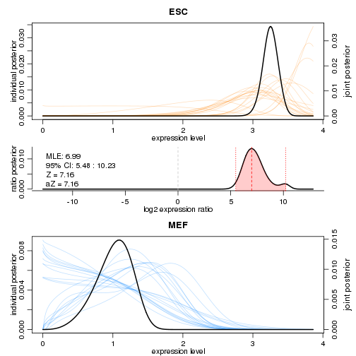
##           lb     mle       ub       ce        Z       cZ
## Tdh 5.482409 6.98927 10.22742 5.482409 7.160813 7.160813
scde.test.gene.expression.difference("Pou5f1",models=scde.fitted.model,counts=counts,prior=scde.prior)
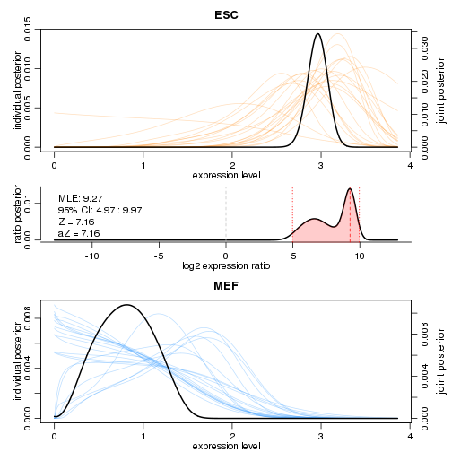
##              lb      mle       ub       ce        Z       cZ
## Pou5f1 4.969435 9.265592 9.970932 4.969435 7.160813 7.160813
On these plots, the coloured curves in the background show the distributions inferred for individual cells, and the dark curves denote overall distributions. By combining information from all the cells, the model is able to infer the overall distribution with high confidence.